Explicability of Artificial Intelligence
Why and for whom?
Artificial Intelligence (AI) makes it possible to harness huge volumes of data to perform complex tasks, usually very efficiently. However, AI models, and more specifically Machine Learning and Deep Learning models, are often compared to “black boxes”, due to their opaque operation, not necessarily understandable by humans. The complexity of these models is therefore a strength, as it enables us to respond to problems better than with simpler models, but it is also a weakness, as it makes them difficult to interpret. However, in certain critical fields such as medical diagnostics or autonomous driving, where human lives may be at stake, control and understanding of the decision-making mechanisms of these models is essential.
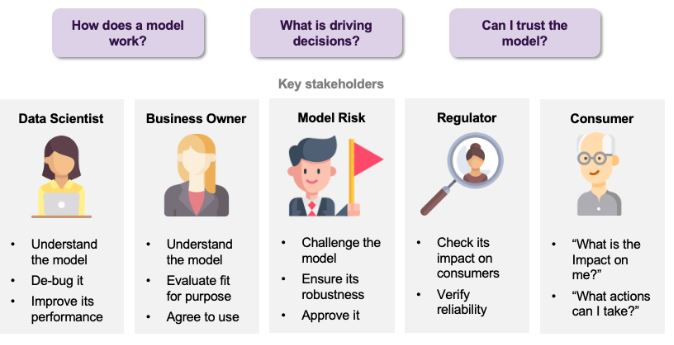
The explicability or interpretability of AI aims to make the operation and results of models more intelligible and transparent to humans, without compromising on performance. This need for explicability concerns different players, each with their own motivations. Firstly, for the Data Scientist who develops the model, a better understanding can help correct certain problems and improve the model. On the business side, explainability can be a means of assessing how well the model matches the company’s strategy and objectives. Explanability can also be used to test the model’s robustness, reliability and potential impact on customers. Finally, it can enable the customer who would be the object of a decision by a system based on an AI model to be informed of the impact of this decision and the potential actions possible to modify it.
With the growing development of artificial intelligence techniques, the question of explicability has become a major challenge for their widespread adoption. Numerous methods of explicability exist and are still being developed today, but certain criteria enable us to distinguish them. Firstly, these methods can have different aims, including explaining a black-box model (post-hoc explicability) or creating an interpretable model (intrinsic explicability), but also verifying the fairness of a model or testing the sensitivity of its predictions. Secondly, the scope of the explanations produced can be local if they concern a particular prediction, or global if they relate to the general behavior of the model. What’s more, some methods are model-specific, while others are model-agnostic, applying to any type of model. Finally, in the same way, a method can be applied to one or more types of data: tabular, images, text…
How does it work?
In order to present a few methods and their application, a simple, concrete example is used: predicting customer churn for a telecom operator. The dataset, Telco Customer Churn [2], comprises around 7,000 customers described by some twenty variables (personal information, services subscribed to, etc.), including churn (yes/no). The problem is therefore one of binary classification on tabular data. Following exploratory analysis and data pre-processing, a Machine Learning model (random forest) is trained on part of the data, the learning sample, and performance evaluation is carried out on the remaining data, the test sample. In order to better understand the decisions made by the model, it is possible to apply explicability methods. The methods presented here are local, so they can be used to explain the model’s decision, whether or not to terminate, concerning a particular customer. The customer chosen to illustrate the different methods is a woman, who has had a monthly contract for just over a year. The model correctly predicted this customer’s termination.
LIME: Local Interpretable Model-agnostic Explanations [3]
One of the most popular explicability methods is LIME (Local Interpretable Model-agnostic Explanations). Its principle is simple: locally approximate the complex model with a simpler, and therefore interpretable, model. This method makes it possible to explain the model’s decision concerning a particular observation, in this case a customer. New instances close to the latter are generated by perturbing the values of the variables. These new instances are weighted according to their proximity to the instance to be explained. Predictions are then made for these new instances. A simple model, such as a linear regression, is finally fitted to these new instances and the associated predictions to produce the explanation.
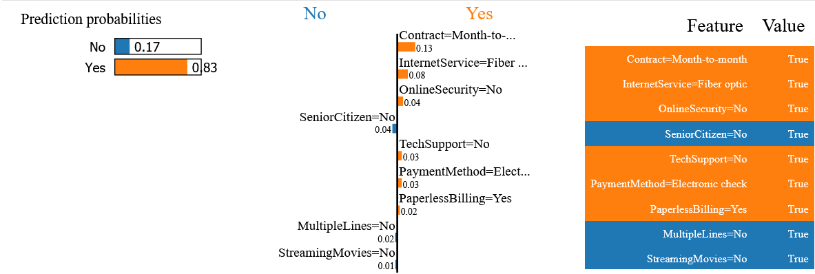
For the chosen customer, the explanation provided by the LIME method indicates that the probability of churn is 83%, and that this prediction is positively influenced by the fact that this customer has taken out a monthly contract with optical fiber.
Anchors [4]
The Anchors method was developed to overcome some of LIME’s problems, in particular concerning the generalizability of explanations, which is not clearly defined. The principle of this second method is to define decision rules that anchor a prediction, using an optimized search algorithm.
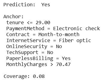
The explanation given for the chosen customer indicates the variables that anchor the churn prediction: a rather low seniority (less than 29 months), a type of electronic payment, a monthly contract, etc. The added value of this method is linked to an additional piece of information, the coverage. In this case, 8% of customers have the characteristics defined by the anchor.
Counterfactual explanations [5]
Unlike the previous method, which focuses on the variables that anchor the predictions, the counterfactual explanations method looks for those whose change would modify the prediction. Several approaches exist to find the smallest possible change that modifies the prediction, including the naive trial-and-error approach or the use of an optimization algorithm. The advantage of this method is that it generates several explanations for a single decision.

Still on the subject of the chosen customer, a first counterfactual explanation consists in the modification of his contract type and payment type. With these two changes, the model predicts non-termination. The same applies if only the customer’s seniority is modified, from 13 to 65 months.
These three methods produce different explanations, but they seem to be consistent with each other, since certain variables are found in all explanations. This is the case for contract type, which appears to be an important factor in prediction. This seems relevant, since it is generally easier to cancel a monthly contract, often without commitment.
What happens next?
This simple use case has illustrated some local explicability methods for a binary classification problem on tabular data. Numerous other methods exist for dealing with different types of problems, models and data. For example, in the field of autonomous driving, some methods can be used to analyze the predictions of an object detector to find out where in the image it is focusing.
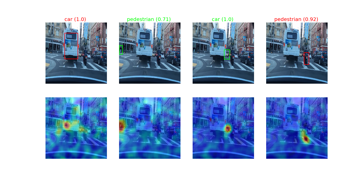
(on the first line: good detection in green, bad detection in red)
In this way, the various explicability methods can be used to identify problems and unexpected behavior in a model, or to compare models with one another. While it is possible to define a strategy for using these explicability methods according to different criteria, it is more complicated to set up a general method for using their results in the testing of AI-based systems. Indeed, AI problems, data and models are diverse. What’s more, expectations in terms of explicability are not necessarily clear-cut (e.g. how do you define the correct behavior of a model without detailed specifications?), and their interpretation may require domain-specific skills.
Finally, explicability methods vary in terms of the techniques used, visualization and type of explanation. One of the difficulties therefore lies in evaluating these methods. However, it is possible to define criteria for comparing them, and to look at their respective advantages and disadvantages. These criteria can be used to select the right method(s) for a given use case. In the context of AI system testing, Kereval is interested in the use of these methods as an additional tool for model analysis.
Related article


